NIFTY over the last 10 years: What the data tells us — and what it can (and can’t) say about 2030

Cdr S Thankappan (Retd), CFP®

Over the past decade, the NIFTY 50 has evolved through multiple market regimes — global liquidity cycles, a once-in-a-century pandemic, rapid digitization, and a structural shift in India’s growth narrative.

Rather than relying on opinions, this article looks at what the last 10 years of data objectively tells us, and how quantitative forecasting models can be used responsibly to think about the road to 2030.

History of NIFTY Index. The NIFTY 50 is the flagship index on the National Stock Exchange of India Ltd. (NSE). The Index tracks the movement of a portfolio of blue-chip companies, the largest and most liquid Indian securities. The Nifty 50 Index represents about 54.10% of the free-float market capitalization of stocks listed on the National Stock Exchange (NSE). The NIFTY 50 has been trading since April 1996 and is owned and managed by India Index Services and Products Ltd (IISL)

Methodology Adopted.         Equity indices are not randomly generated values instead they can be treated as a discrete-time series model which is based on a set of well-defined numerical data items collected at successive points at regular intervals of time. We shall develop and use different models to predict NIFTY. Forecasts are done under the assumption that the market and other conditions in future would continue to be very much like the present. Not that there would be no changes, but that the change if at all would be gradual, not a drastic one.

Data. Data set used here is obtained from the archives of the NSE url <<NSE - National Stock Exchange of India Ltd. (nseindia.com)>>. The dataset has collated information regarding the daily NIFTY index values. The data used comprises of daily NIFTY adjusted close values during the period from 01 Jan 2016 till 09 Jan 2026. Next step mainly consists of cleaning the dataset, looking for and imputing null values, finding duplicate data points and getting rid of them. Next, we parse date values and make the dataset ready for time series analysis. The python script for the forecasting study could be found at the link below.

NIFTY_FORECAST_2030.ipynb - Colab

Part 1: What the last 10 years reveal

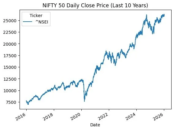
Past Price Variations. The NIFTY index has passed through a turbulent past ten-year period, although with a clear upward trend. A plot of the variation is as shown below:

Yearly Box Plot.        There is a clear uptrend visible across the years, with major volatility visible in 2020 due to the onset of pandemic.

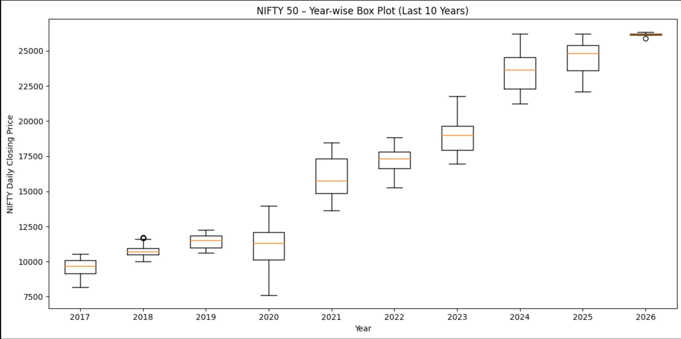
Following inferences can be made from the above plot:

Median trend (orange line in each box)

·        Clear structural upward shift in medians year after year

·        Indicates strong long-term trend component → trend-stationarity issues if not differenced

Box height (IQR = volatility)

·        2020 shows a very wide IQR → COVID shock & regime break

·        2021–2023: elevated but more stable volatility

·        2024–2026: volatility compressing despite higher levels → late-cycle behavior

Whiskers & outliers

·        Long lower whisker in 2020 → downside tail risk

·        Fewer extreme outliers in recent years → market maturity & liquidity effect

Monthly Box Plot.     There is absolutely no seasonality present in the data.

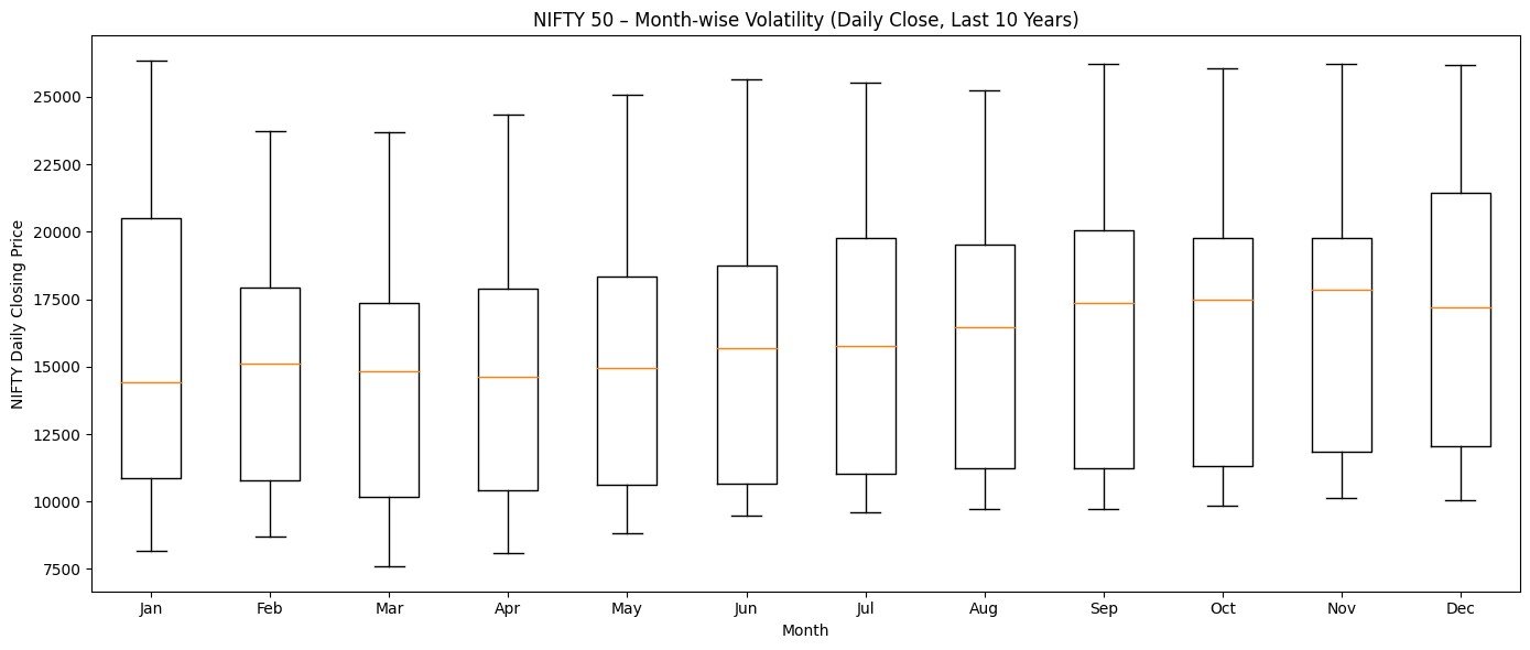
Key insights from the monthly box plot

🔹 High-volatility months

·        March - Widest IQR and long whiskers, consistent with financial year-end flows, global risk repricing

·        October - Elevated volatility due earnings season + global macro events

·        June - Noticeable spread, often influenced by global risk cycles and policy expectations

🔹 Relatively stable months

·        December - Narrower IQR → lower volatility. Typically, year-end positioning and liquidity effects

·        August - Moderately compressed distributions

🔹 Skewness & tail risk

·        Several months show upper-tail skew → strong upside momentum phases

·        Downside tails cluster more in Mar–Apr, indicating drawdown risk

Monthly index variations across the years.               A plot of monthly index variations for the various years under consideration is shown below.

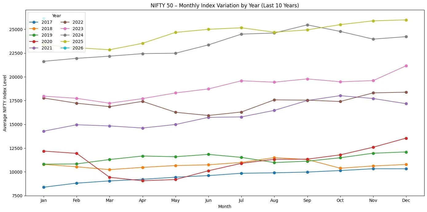
Key insights from the monthly variation plot:

Strong seasonality across years

·        Jan–Mar: frequent softness or consolidation

·        Jul–Sep: consistent upward bias

·        Oct–Dec: strongest momentum phase in most years

This aligns well with earnings cycles, liquidity & institutional flows and festive / year-end positioning

Regime shock clearly visible in 2020 as the line shows a sharp breakdown in Mar–Apr and a fast recovery from mid-year onward. This visually confirms non-linear behavior, critical for model selection

Trend persistence in recent years

·        2023–2026 show higher base levels and smoother monthly transitions, which indicates reduced downside volatility and strong trend dominance → momentum-friendly regime.

Trend & Seasonality.            A decomposition plot of the timeseries data is plotted below. The trend curve gives an impression of steadily increasing trend across the years. While absence of seasonality pattern is evident from the seasonality curve, lots of error/residuals (white noise) are present.

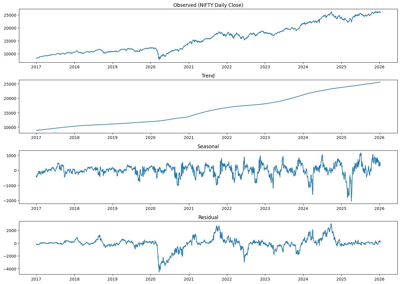
Key insights from the Decomposition Plot:

Observed - NIFTY index clearly shows a long-term uptrend, with a sharp COVID drawdown and a post-2020 structural acceleration.

Trend (most important for forecasting) - Is smooth, non-linear upward trajectory. The trend slope steepens after 2020, indicating a regime change which confirms that the series is non-stationary

Seasonal component - Captures recurring intra-year patterns, where the seasonal amplitude increases with index level. This reflects earnings cycles, FII/DII flow seasonality and calendar effects identified earlier (Mar, Oct volatility)

Residual (noise + shocks) - Large negative spike in early 2020 (black swan). Volatility clustering persists → not white noise.  Post-2022 residuals are smaller.

Conclusion to Part 1: What the Last 10 Years Reveal

A Strong, Persistent Long-Term Trend - Daily closing price data over the past decade shows a clear upward trend, interrupted by short but sharp drawdowns. One can safely conclude that the the index is non-stationary — it does not revert to a long-term mean. Any model assuming “average” behaviour (simple mean, static expectations) fails badly. This confirms a fundamental truth about equity indices: They compound, they don’t oscillate.

Volatility Is Not Constant - Year-wise and month-wise analysis highlights that 2020 was a structural break (COVID shock) and that the volatility, though elevated, stabilised post-2021. Certain months (notably March and October) repeatedly showed higher dispersion.

Seasonality Exists — But It’s Subtle - STL (Seasonal-Trend decomposition) showed a recurring intra-year pattern. Seasonality, though small relative to trend, was however statistically present.

Part 2: What Simple Models Teach Us (Before Using Complex Ones)

Train-Test Split. We divide the data into train and test data. Train data comprises all the data points till 31 Dec 2022 and test dataset comprises of all the balance data points. This split is considered most optimum since it is both time-aware and regime-sensitive (especially since it includes the data from pre-COVID, COVID shock and early post-COVID recovery phases.

Model Building.        Next we build various models such as regression model (LR), naïve forecast model, simple average model (SA) and exponential smoothing model on the training data and evaluate the model using RMSE on the test data. The performance of the models on test data are indicated below in the plots. In exponential smoothing model we choose Double Exponential (Holt’s) Model based on the assessment that, while level and trend are available in the data, seasonality is missing.

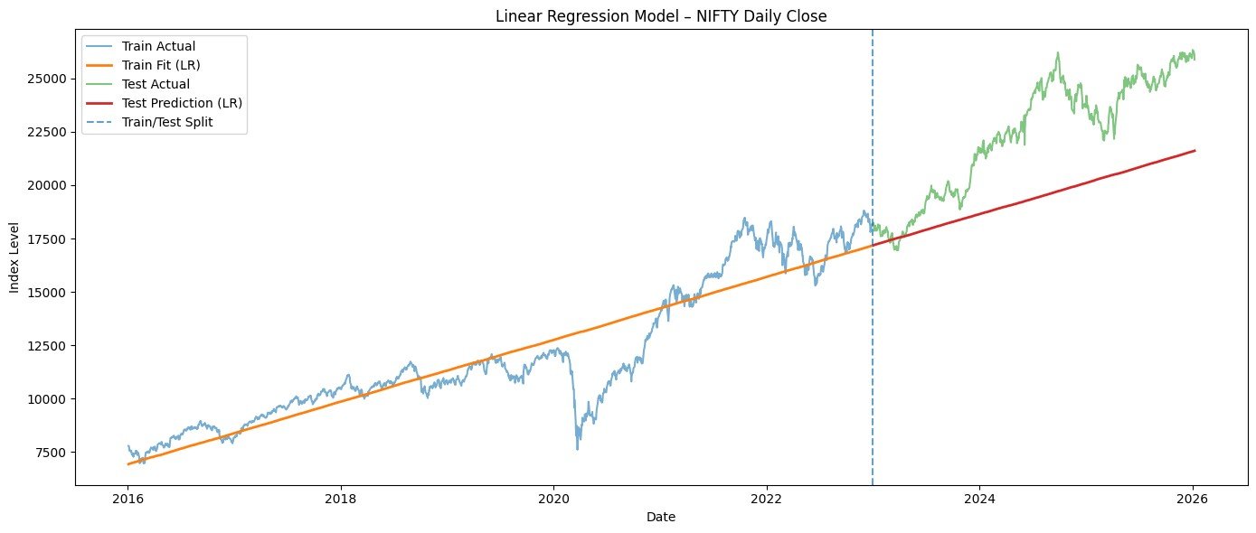
What LR Model tells us - The regression uses time as the only feature, and it effectively fits a straight-line trend through the training period. This makes LR a trend benchmark, not a forecasting model. LR fits the average long-term trend reasonably well in-sample but fails to capture cycles, seasonality, volatility clustering and post-2023 trend acceleration. In the test period, LR systematically underestimates the index and shows large bias → classic structural break effect.

This is expected and actually useful diagnostically, since this forms a baseline benchmark. Any serious model must beat this LR line on RMSE / directional accuracy / drawdown behavior. 

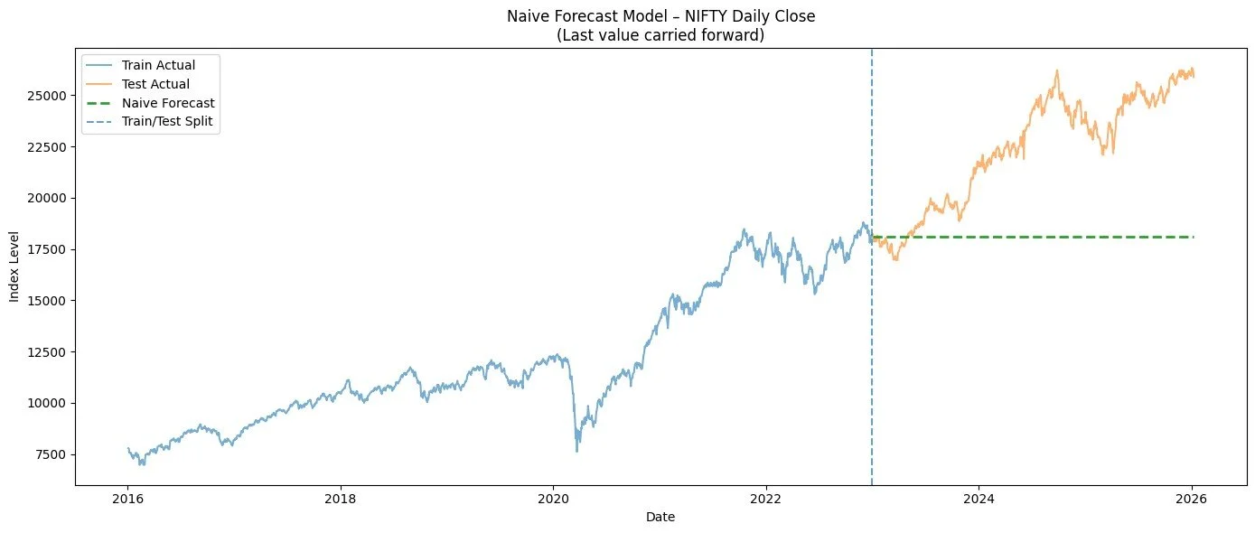
What the Naive Model tells us - Post-2022, NIFTY enters a strong upward regime. The naive forecast stays flat and severely underestimates the index. It accumulates large systematic error. This confirms strong trend persistence and high opportunity cost of static models. However, this is useful in benchmarking. Any model we build must beat the naive forecast on RMSE / directional accuracy / cumulative forecast error. If it doesn’t → the model has no economic value.

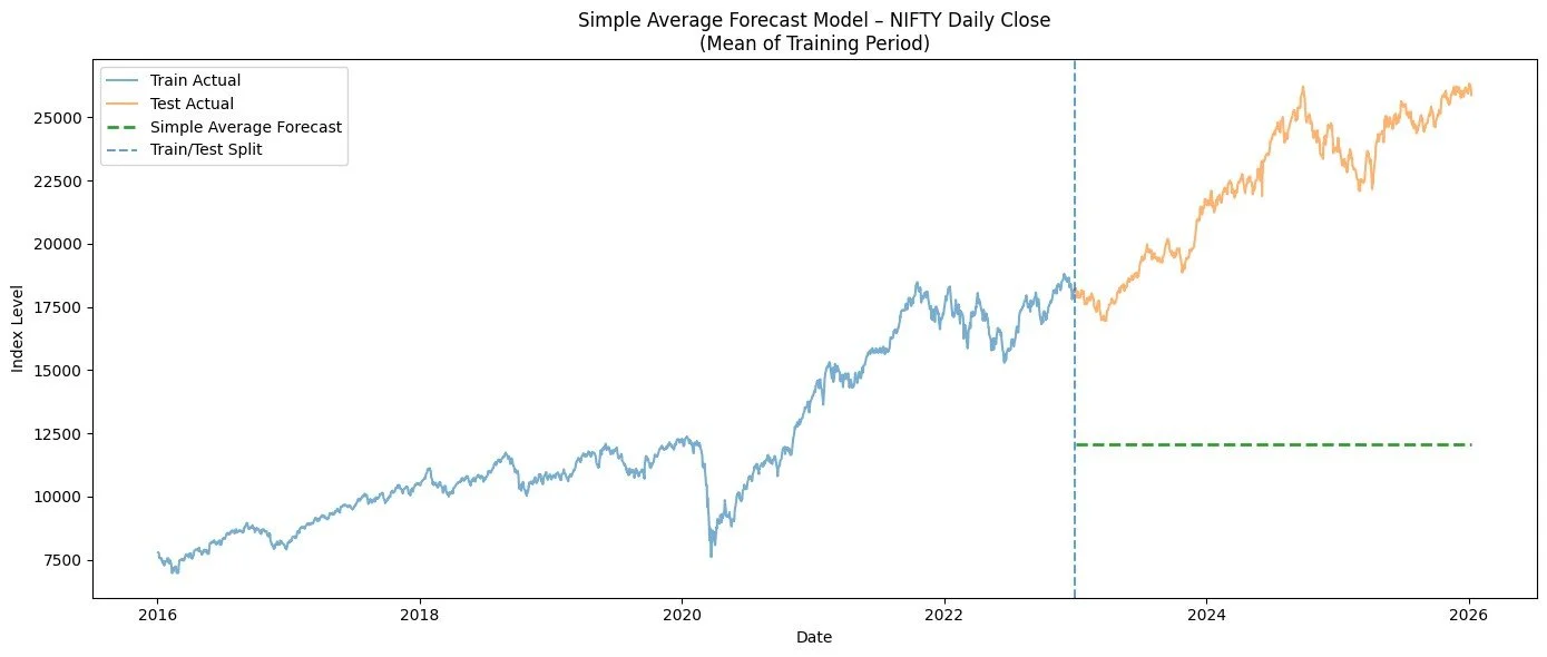
What SA Model tells us - The series fluctuates around a constant mean. It has no trend, no seasonality, no memory. This assumption is completely violated for equity indices. The plot clearly shows that the average forecast sits far below the test-period actuals. The error increases monotonically over time. Bias is worse than the Naive (last value) model. This is expected because markets trend upward over long horizons and historical averages become irrelevant in trending regimes.

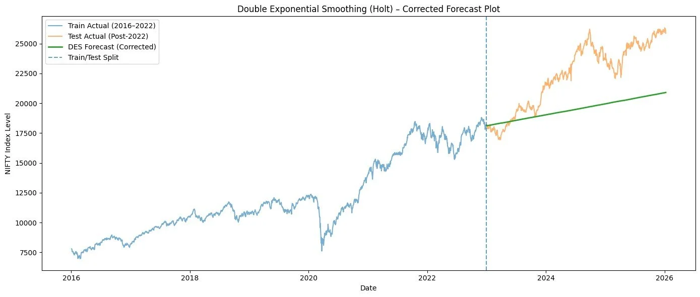
What DES Model tells us - It captures level and trend, while omitting seasonality and regime breaks. This already makes DES strictly superior to Naive, Simple Average and Plain Linear Regression (in most cases). In the present instance, DES learns the pre-2023 trend slope and projects it forward smoothly. In the test period, it performs much better than Naive / Average but still underestimates the sharp post-2023 acceleration. This is what we expect, since Holt assumes trend persistence, but markets experienced trend steepening.

Model Errors - The RMSE values for the models (errors between the predicted values and the test values) are indicated below.

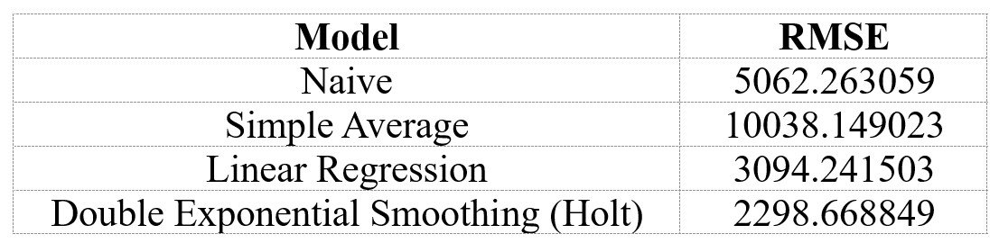
Best performer: Double Exponential Smoothing (Holt) - Lowest RMSE on this test window and more stable than LR in general. Often preferred in production due to smoother behavior and less sensitivity to noise. The close second is Linear Regression, which has slightly higher RMSE than DES. It indicates strong trend dominance post-2022, due to which linear trend extrapolation worked well. Baselines behaved as expected. Naive beat Simple Average, confirming trend persistence.

What this tells you about the market regime - 2023–2025 is a strong trending regime. Models that explicitly learn trend → perform well and those which assume stationarity → fail badly. This is exactly what our earlier decomposition plot suggested. 

Conclusion to Part 2: What Simple Models Teach Us (Before Using Complex Ones)

Before jumping to advanced forecasting, it’s critical to establish benchmarks.

When tested on post-2022 data:

• Naive model (last value) → underestimates strongly trending markets

• Simple average model → performs worst (assumes mean reversion)

• Linear regression → captures trend but breaks under regime change

• Double exponential smoothing (Holt) → smoother, more realistic trend tracking

Lesson: If advanced models cannot beat these baselines, it has no economic value.

Part 3: Forecasting NIFTY Till 2030 — The Right Way to Think About It

Predictions till 2030.             Now we prepare the prediction dataset by parsing dates after 2026 till 2030. This prediction dataset is used on two of the previously developed and trained models (LR and Holt’s/DES Models). We additionally use the timeseries model for the prediction. The plots of predictions are included below.

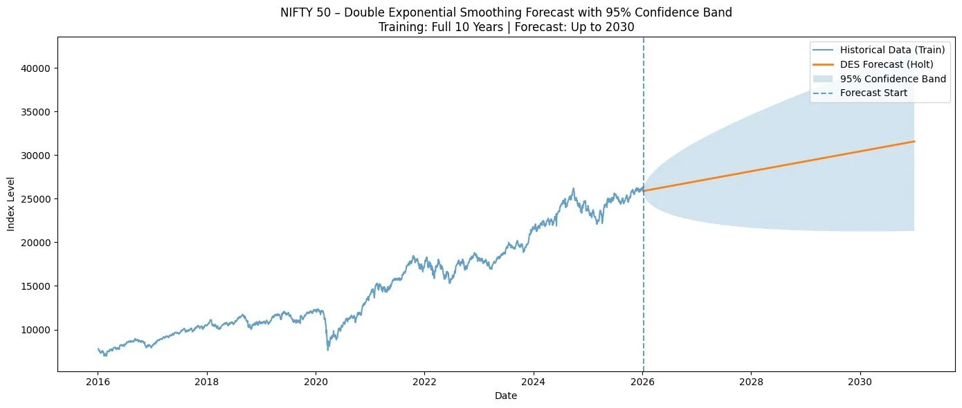
What DES forecast tells us - It is a trend extrapolation, not a price target. Holt assumes that the trend learned from the last 10 years continues and there are no structural breaks or explicit seasonality. So read this as: “If the long-term trend observed over the past decade persists, this is the implied trajectory.” DES forecast is useful for Strategic planning, Long-horizon expectations and Scenario baselining. It is not suitable for short-term trading decisions. The confidence band represents an approximate forecast uncertainty band, derived from in-sample residual volatility and error accumulation growing with √h (forecast horizon). Unlike LR, DES reacts more smoothly to recent trend and produces a more conservative central path. But it still shows rapidly expanding uncertainty beyond 2–3 years.

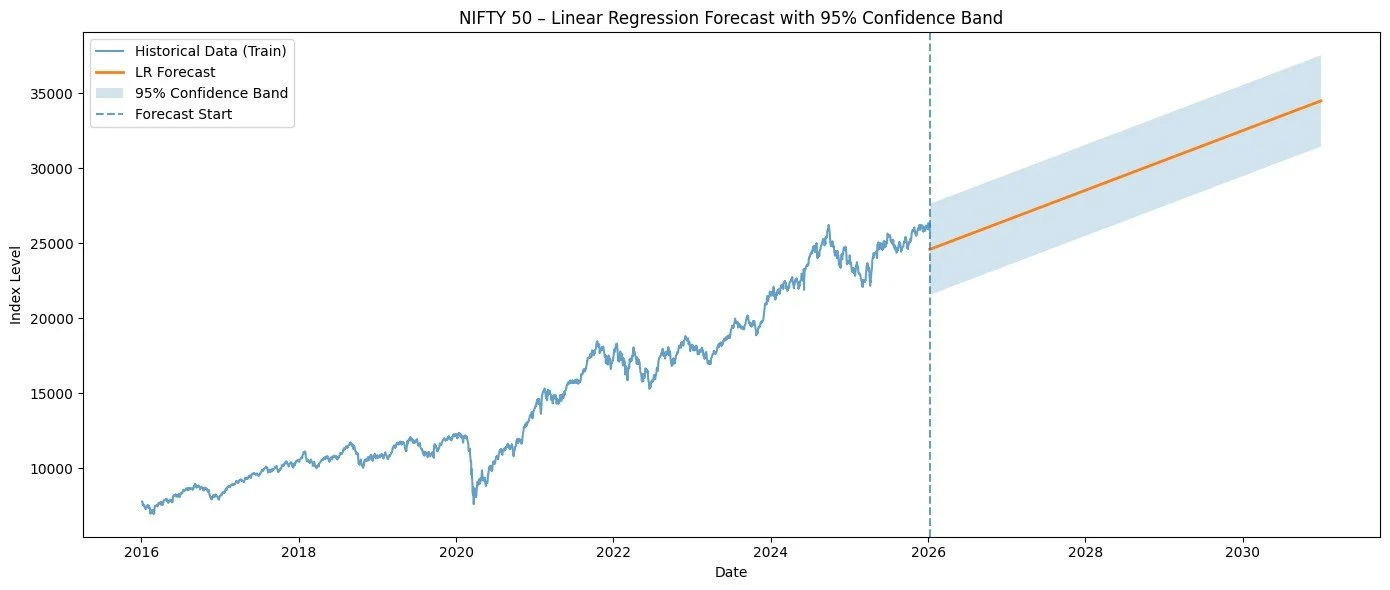
What LR forecast tells us - It uses time as the only explanatory variable and fits a single straight-line trend over the full 10 years. It then projects that slope forward until 2030. The band represents a statistical confidence interval for the conditional mean, not a guarantee of future prices. It reflects historical volatility of residuals and increasing uncertainty as the horizon extends. That’s why the band fans out as we move toward 2030. By 2028–2030, the confidence range is very wide and this visually communicates why long-term index forecasting is fragile. The central LR line assumes one constant growth rate and no regime shifts. Real markets will almost certainly move in and out of this band.  

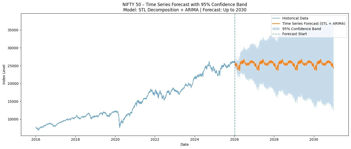
What Time Series (STL + ARIMA) Forecast tells us - It handles trend and seasonality and produces statistically grounded confidence intervals. It is more realistic in medium-term behavior. The band widens because forecast error accumulates over time and the structural uncertainty increases with horizon.

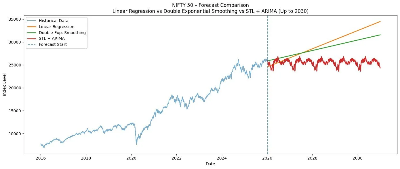
 How to read this comparison

Shape & aggressiveness

·        LR is the most aggressive (single constant slope).

·        DES (Holt) is smoother and typically more conservative than LR.

·        STL + ARIMA adapts to recent dynamics and seasonality; often most realistic mid-term.

Model suitability by horizon

·        Short–medium term (months to ~1–2 years): STL + ARIMA

·        Medium term (trend continuation): DES (Holt)

·        Long-term scenario baseline: LR (use with wide uncertainty bands)

Practical takeaway

If one has to pick one classical model for planning and communication, STL + ARIMA is the best-balanced choice; use DES as a conservative cross-check and LR as a trend scenario.

Conclusion to Part 3: Forecasting NIFTY Till 2030 — The Right Way to Think About It

Using the above tools, we model the long-term trend, seasonality and short-term dynamics. This approach produces a central forecast path and a 95% confidence band that widens meaningfully with time. The forecast tells us the long-term direction remains upward and that the uncertainty increases dramatically beyond 2–3 years. By 2030, the confidence range is wide — not because the model is weak, but because reality is uncertain.

What It Does Not Tell Us

• It does not predict crashes

• It does not account for valuation extremes

• It does not guarantee outcomes

In other words:

This is a scenario map, not a price target.